
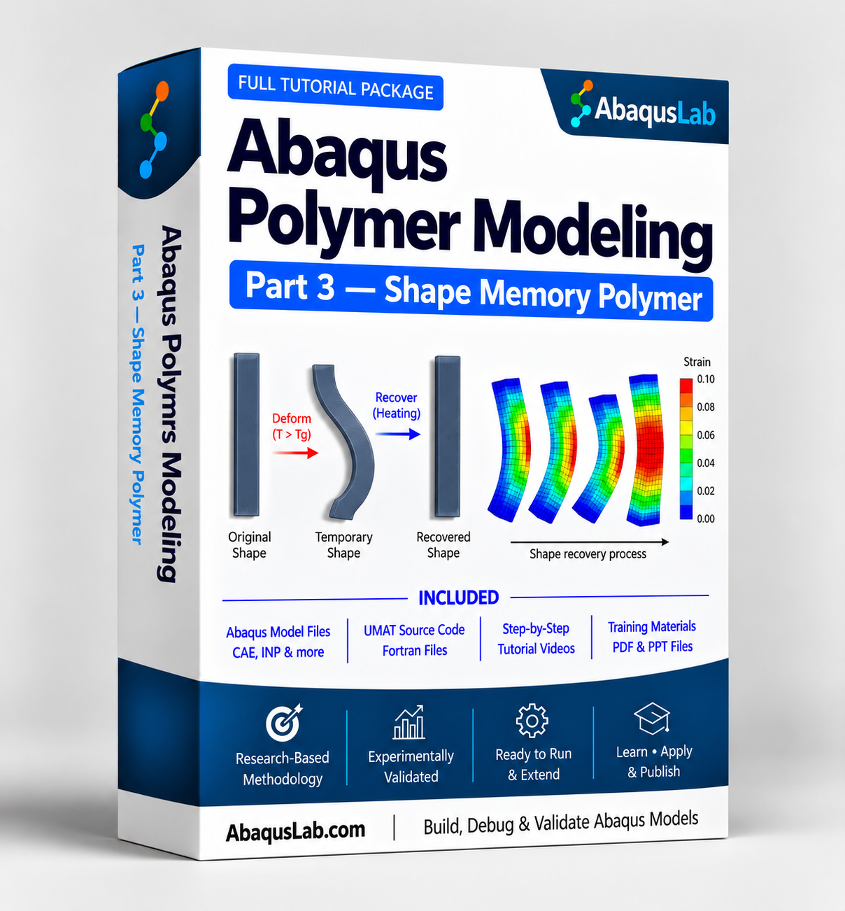


Description
Abaqus Shape Memory Polymer VUMAT | Thermomechanical Modeling
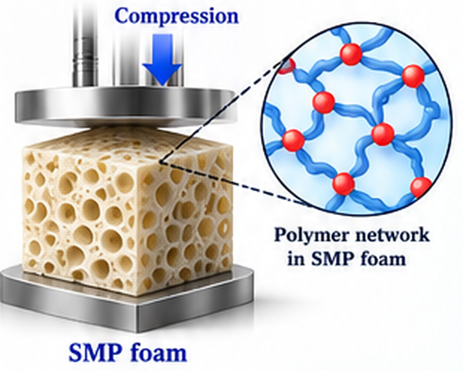
This comprehensive Abaqus shape memory polymer tutorial presents shape memory polymer VUMAT development and SMP Abaqus simulation using a finite-strain thermo-visco-plastic model in Abaqus/Explicit. The thermomechanical polymer Abaqus formulation combines Arruda–Boyce hyperelasticity, Eyring viscous flow, temperature-dependent deformation, and glass-transition behavior. This Abaqus thermomechanical polymer and thermo viscoplastic VUMAT tutorial covers shape memory polymer simulation, shape memory polymer foam compression, structural relaxation, fictive temperature, and strain-rate effects.
This tutorial builds on two peer-reviewed shape memory polymer studies: Jarrah et al. (2021), published in Actuators, and Nguyen et al. (2008), published in Journal of the Mechanics and Physics of Solids. The tutorial combines the thermo-visco-plastic SMP foam modeling framework of Jarrah et al. with the structural relaxation and fictive-temperature theory of Nguyen et al., adapting these related but distinct formulations into a practical Abaqus/Explicit VUMAT tutorial.
What Is Abaqus Shape Memory Polymer Modeling and How Does an SMP VUMAT Work?
Abaqus polymer modeling is the finite element simulation of polymer materials under mechanical loading, including nonlinear deformation, strain-rate sensitivity, yielding, strain softening, and strain hardening. An Abaqus polymer VUMAT enables researchers to implement custom constitutive models in Abaqus/Explicit using Fortran. Part 3 focuses on a shape memory polymer VUMAT with thermal deformation, an eight-chain equilibrium network, Eyring viscous flow, and temperature-dependent SMP foam compression.
Why Use a Shape Memory Polymer VUMAT for Thermomechanical Polymer Abaqus?
The shape memory polymer VUMAT combines an equilibrium eight-chain network with a nonequilibrium viscous branch. Thermal and mechanical deformation are separated, and temperature-dependent viscous flow captures the sensitivity of SMP foam compression to loading rate and temperature.
How Does Eyring Flow Capture Temperature- and Rate-Dependent SMP Behavior?
Eyring viscous flow uses a hyperbolic-sine stress activation law. Temperature and the polymer relaxation state affect molecular mobility, while the deviatoric driving stress determines the viscous deformation rate.
How Do Temperature and Strain Rate Affect SMP Abaqus Simulations?
SMP Abaqus analysis evaluates compression curves at different prescribed temperatures and strain rates. Glass transition changes molecular mobility and relaxation, while Eyring flow introduces stress-activated rate sensitivity. Compression validation does not itself verify a complete shape-recovery cycle.
Shape Memory Polymer VUMAT Model and Governing Equations
The SMP formulation separates thermal and mechanical deformation and combines an equilibrium Arruda–Boyce eight-chain network with a nonequilibrium Eyring viscous response. The primary VUMAT foam-compression formulation follows Jarrah et al. (2021); the complementary fictive-temperature and structural-relaxation theory follows Nguyen et al. (2008).
1. Thermo-Visco-Plastic Constitutive Model
The SMP model combines an elastic–viscous nonequilibrium branch with an Arruda–Boyce hyperelastic network. Their stresses add in parallel, while the series elements of the nonequilibrium branch carry equal stress (Jarrah et al., Eqs. 4–7).
Total stress
\boldsymbol{\sigma}_p=\boldsymbol{\sigma}_p^{e}+\boldsymbol{\sigma}_p^{he}
\]
\boldsymbol{\sigma}_p^{ve}=\boldsymbol{\sigma}_p^{e}=\boldsymbol{\sigma}_p^{v}
\]
- Finite-strain kinematics
- Arruda–Boyce rubbery network
- Eyring temperature-dependent flow
- PU and styrene SMP foam compression
2. Finite-Strain Elastic Stress and Thermal Strain
The glassy elastic branch uses a logarithmic elastic strain with a thermal correction. The elastic modulus tensor is defined using the glassy shear modulus and Lamé constant (Jarrah et al., Eq. 8).
\boldsymbol{\sigma}_p^{e}=\frac{1}{J_p^{e}}\,\mathbb L_p^{e}:\left[\ln\mathbf F_p^{e}-\frac{\alpha_r+\alpha_g}{2}(T-T_0)\mathbf I\right]
\]
\(\mathbf F_p^e\) : elastic deformation gradient
\(G_p\) : glassy shear modulus
\(\lambda_p\) : Lamé constant
\mathbb L_p^e=2G_p\mathbb I_4+\lambda_p\mathbf I\otimes\mathbf I
\]
J_p^e=\det(\mathbf F_p^e)
\]
3. Arruda–Boyce Hyperelastic Network
The Arruda–Boyce eight-chain spring describes the nonlinear rubbery stress and finite-chain locking at large deformation (Jarrah et al., Eq. 9).

Chain stretch
\lambda_{\mathrm{chain}}=\sqrt{\frac{\operatorname{tr}(\overline{\mathbf B})}{3}}
\]
Rubbery network stress
\boldsymbol{\sigma}_p^{he}=\frac{1}{J_p^{he}}\left[\mu_r\frac{\lambda_L}{\lambda_{\mathrm{chain}}}\mathcal L^{-1}\!\left(\frac{\lambda_{\mathrm{chain}}}{\lambda_L}\right)\overline{\mathbf B}^{\,\prime}+k_b(J_p^{he}-1)\mathbf I\right]
\]
Langevin function
\mathcal L(\beta)=\coth\beta-\frac{1}{\beta}
\]
4. Temperature-Dependent Eyring Flow
The Eyring dashpot captures thermally activated viscous shear flow. Its rate depends on shear stress, glass-transition temperature, fictive temperature, and athermal shear strength (Jarrah et al., Eqs. 10–11).
\mathbf D^v=\dot\gamma^v\mathbf n\qquad\dot\gamma^v=\frac{sT}{\eta_g Q}\exp\!\left[C_1\frac{C_2(T-T_f)+T(T_f-T_g)}{T(C_2+T-T_g)}\right]\sinh\!\left(\frac{\tau Q}{sT}\right)
\]
\(\mathbf D^v\) : viscous deformation-rate tensor, \(\mathbf n\) : normalized flow direction, \(\dot\gamma^v\) : viscous shear strain rate, \(T_f,T_g\) : fictive and glass-transition temperatures, \(\eta_g,Q,C_1,C_2\) : glass-transition viscosity, activation parameter, and WLF constants
Equivalent shear stress
\tau=\frac{1}{2}\left\|\operatorname{dev}\boldsymbol{\sigma}_p^e\right\|
\]
\(\tau\) : effective shear stress \(s\) : athermal shear strength
5. Fictive Temperature and Structural Relaxation
Nguyen et al. (2008) describe the nonequilibrium polymer structure through a fictive temperature that relaxes toward the actual temperature. This relation provides complementary thermal-recovery theory, not a separate claim of VUMAT validation.
\frac{dT_f}{dt}=-\frac{T_f-T}{\tau_R}
\]
\(T_f\) : fictive temperature, \(T\) : actual material temperature, \(\tau_R\) : structural relaxation time
Thermal history and relaxation

6. Thermal and Mechanical Deformation Gradients
The total deformation gradient separates into mechanical and thermal parts, while the viscoelastic mechanical branch is decomposed further into elastic and viscous gradients (Jarrah et al., Eqs. 1–2, 6–7).
\mathbf F
=
\mathbf F_M\mathbf F_T
\]
\(\mathbf F\) : total deformation gradient
\(\mathbf F_M\) : mechanical deformation
\(\mathbf F_T\) : isotropic thermal deformation
\mathbf F_p^{ve}=\mathbf F_p^e\mathbf F_p^v
\]
\mathbf F_T
=
J_T^{1/3}\mathbf I
\]
7. Thermomechanical VUMAT Integration Algorithm
The SMP foam VUMAT uses a midpoint Runge–Kutta scheme to integrate the viscous response and update stresses and state variables at Abaqus/Explicit integration points (Jarrah et al., Section 2.3).
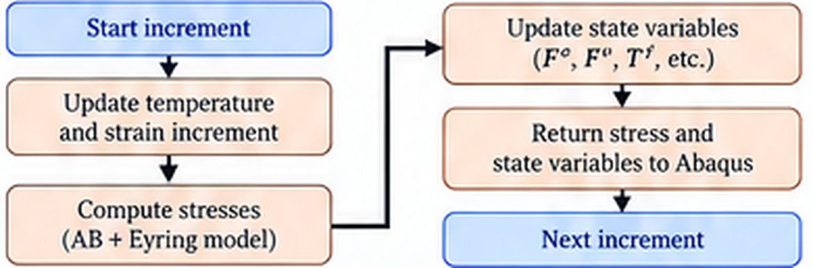
- Midpoint integration scheme for stability and accuracy
- Update mechanical and thermal deformation, elastic and rubbery stress, viscous flow, and state variables
- Implemented in Abaqus/Explicit using VUMAT subroutine
8. Temperature-Dependent SMP Foam Results
The polyurethane and styrene SMP foam compression simulations demonstrate temperature- and rate-sensitive stiffness, yielding, softening plateaus, and densification (Jarrah et al., 2021). They do not independently validate a complete shape-recovery cycle.

Required Prerequisites for Shape Memory Polymer VUMAT
Complete Polymer Parts 1 & 2 Before Advanced Shape Memory Polymer Modeling
Polymer Part 1 — Abaqus VUMAT Fundamentals introduces Fortran programming, the VUMAT interface, stress-update algorithms, and state-variable management in Abaqus/Explicit.
Polymer Part 2 — Arruda–Boyce VUMAT develops finite-strain polymer constitutive modeling, eight-chain hyperelasticity, viscoplastic flow, and numerical integration. These concepts provide the essential foundation for the temperature-dependent, thermo-visco-plastic shape memory polymer VUMAT developed in Part 3.
Required learning sequence:
Fortran programming → VUMAT interface → stress updates → state variables → Abaqus/Explicit
Finite-strain kinematics → eight-chain hyperelasticity → viscoplastic flow → numerical integration
Thermal deformation → temperature-dependent Eyring flow → SMP foam compression → thermomechanical analysis
What Does the Abaqus Shape Memory Polymer VUMAT Tutorial Cover?
This Abaqus shape memory polymer tutorial covers finite-strain thermomechanics, thermal deformation, eight-chain network elasticity, Eyring flow, fictive-temperature theory and SMP foam compression.
Shape Memory Polymer VUMAT
User-defined constitutive behavior in Abaqus/Explicit.
Large-Deformation Polymer Mechanics
Deformation gradients and finite-strain kinematics.
Thermal Deformation Gradient
Logarithmic strain and numerical approximations.
Eight-Chain Polymer Network
Langevin backstress and limiting chain stretch.
Eyring Thermo-Viscoplastic Flow
Rate-sensitive inelastic flow and material softening.
Temperature and Rate Sensitivity
Loading-rate effects on yield and deformation.
Midpoint Stress Integration
Incremental numerical updates and error control.
Fortran VUMAT Implementation
Stress arrays, material parameters, and state variables.
Glass Transition and Relaxation
Evolution of the internal shear-strength variable.
Fictive Temperature Evolution
Molecular-chain alignment and network resistance.
SMP Compression Verification
Parameter sensitivity and numerical consistency.
Thermomechanical Compression
Comparison of stress–strain response and hysteresis.
Abaqus Shape Memory Polymer Learning Path — Parts 1–3
The AbaqusLab Polymer VUMAT Series begins with VUMAT programming fundamentals in Part 1, advances to Arruda–Boyce viscoplastic polymer modeling in Part 2, and extends to thermomechanical shape memory polymers in Part 3. Recommended study order: Part 1 → Part 2 → Part 3. Advanced parts may also be studied independently by experienced VUMAT users.
Part 1 — Abaqus VUMAT Fundamentals
- ⚙️ VUMAT subroutine fundamentals
- 💻 Fortran implementation
- 📐 Stress updates and state variables
- 🔍 Practical Fortran examples
£99 Student: £59
Part 2 — Arruda–Boyce Polymer VUMAT
- 📘 Finite-strain polymer mechanics
- ⚙️ Eight-chain Arruda–Boyce model
- 📊 Strain-rate and softening effects
- 📉 Polymer hardening and backstress
£179 Student: £119
Part 3 — Shape Memory Polymer VUMAT
- 💻 Shape memory VUMAT formulation
- ⚙️ Thermomechanical material response
- 📊 Programming and recovery behavior
- 🔄 Shape fixing and recovery
£229 Student: £149
Complete Abaqus Polymer VUMAT Modeling Suite — Parts 1–3
- Complete Parts 1–3 learning path
- VUMAT Fortran programming
- Polymer constitutive equations and integration
- Arruda–Boyce eight-chain network
- Rate-dependent viscoplastic response
- Shape memory polymer formulation
- Thermomechanical shape recovery
- Progressive polymer modeling tutorials
What You Receive with This Abaqus Shape Memory Polymer VUMAT Tutorial
This Abaqus Shape Memory Polymer Tutorial is designed as a learning and implementation package. You receive Abaqus models and shape memory polymer VUMAT source code, step-by-step tutorial videos, constitutive formulation explanations, supporting files, documentation, and technical support required to understand, run, modify, and extend the viscoplastic polymer Abaqus workflow, including Abaqus polymer VUMAT implementation and Abaqus strain rate polymer analysis.
Complete Step-by-Step Tutorial Videos
▶ Complete Abaqus Shape Memory Polymer VUMAT video training
VUMAT, Abaqus Models, Tutorials & Support
Package objective:
The goal is not only to provide a working Shape Memory Polymer VUMAT, but to give you a complete and reusable Abaqus polymer modeling and viscoplastic polymer simulation workflow that you can understand, verify, modify, and extend for your own material modeling, research, and engineering applications.
Abaqus Shape Memory Polymer VUMAT — Thermomechanical Learning Sequence
From Polymer Constitutive Theory to VUMAT Implementation
The learning sequence progresses from thermal and finite-strain polymer mechanics to the shape memory polymer VUMAT formulation, Fortran implementation, and stress–strain verification.
Abaqus Shape Memory Polymer and VUMAT Subroutine Workflow
A practical Abaqus polymer modeling workflow combines finite-strain constitutive equations, Fortran VUMAT implementation, parameter studies, and independent numerical verification.
What You Will Learn with the Abaqus Shape Memory Polymer VUMAT Tutorial
Understand Abaqus Polymer Modeling
Explain nonlinear polymer deformation, rate dependence, and chain hardening.
Build an Abaqus Polymer Simulation
Connect material parameters, loading rates, and stress–strain response.
Develop a VUMAT Polymer Subroutine
Implement elastic stress, viscoplastic flow, and network backstress.
Predict Polymer Deformation Abaqus
Evaluate large deformation and nonlinear stress–strain behavior.
Model Strain-Rate-Dependent Polymer Response
Relate flow parameters to yielding, strain softening, and hardening.
Explore Glass-Transition Parameters
Examine rubber modulus, limiting chain stretch, and flow parameters.
Interpret Eyring Flow and Network Elasticity
Study chain stretch, backstress, and large-strain strengthening.
Validate Polymer Finite Element Results
Assess deformation and density against measurements.
Who Is This Abaqus Shape Memory Polymer VUMAT Tutorial For?
- Researchers studying nonlinear and rate-dependent polymer behavior
- Engineers investigating polymer yielding, softening, and hardening
- Finite element analysts developing custom VUMAT models
- Researchers implementing Arruda–Boyce constitutive equations
- PhD and MSc students in computational polymer mechanics
- Fortran developers implementing finite-strain VUMAT routines
- Engineers assessing strain-rate effects in polymer deformation
- Abaqus/Explicit users progressing beyond conventional polymer models
Need Custom Abaqus Shape Memory Polymer Modeling or VUMAT Development?
Custom Abaqus polymer modeling can require experimental calibration of viscoplastic flow parameters, network hardening, strain softening, and finite-strain stress integration. AbaqusLab provides consulting for advanced Abaqus/Explicit modeling, user subroutines, and numerical verification.
Abaqus Shape Memory Polymer — Frequently Asked Questions
What is a shape memory polymer VUMAT?
A Fortran user-material subroutine that computes polymer stress and state-variable updates in Abaqus/Explicit.
Is this SMP formulation temperature- and strain-rate-dependent?
Yes. The Jarrah et al. (2021) SMP foam VUMAT uses temperature-sensitive constitutive behavior and an Eyring-type viscous flow response to predict compression at different temperatures and rates.
How does the model represent SMP network elasticity?
An Arruda–Boyce eight-chain network represents equilibrium hyperelasticity, alongside a nonequilibrium branch for time-dependent response.
What numerical integration method is discussed?
The Jarrah et al. (2021) SMP foam formulation discusses midpoint Runge–Kutta time integration of constitutive variables.
Why is thermal deformation gradient decomposition important?
The split F = F_M F_T separates thermal expansion from mechanical deformation; the mechanical part is then split into elastic and viscous components.
Can temperature and strain-rate effects be studied in Abaqus?
Yes. Simulations can compare SMP foam compression responses at different prescribed temperatures and strain rates.
Is Part 1 required?
Part 1 is recommended for VUMAT fundamentals, while Part 2 introduces eight-chain polymer constitutive modeling.
Is a full thermal shape-recovery cycle validated?
No. Temperature-dependent foam compression and complete thermal shape recovery are different validation problems. Nguyen et al. (2008) provides a recovery-oriented framework, but it should not be conflated with the Jarrah et al. (2021) compression VUMAT.
Related Abaqus Polymer VUMAT, Material Modeling & Advanced Simulation Resources
Continue studying Abaqus polymer VUMAT, Abaqus VUMAT subroutine development, nonlinear polymer mechanics, and advanced finite element simulation through related AbaqusLab tutorials and research resources. These learning paths connect polymer constitutive modeling with composite damage, impact, cutting, soil deformation, wear simulation, fracture mechanics, hydrogen transport, and microstructure-sensitive material modeling.
1
RELATED COMPOSITES TUTORIALS
Study progressive damage, composite failure, impact and machining using VUMAT in Abaqus/Explicit.
Composite Impact & Progressive Damage VUMAT
- Laminate impact simulation
- Progressive composite damage
- VUMAT implementation
CFRP Cutting & Damage VUMAT
- CFRP cutting simulation
- Fiber orientation effects
- Material removal and damage
2
RELATED SOIL MODELING TUTORIALS
Explore large deformation, penetration and rate-dependent soil behavior using CEL and VUMAT.
Abaqus CEL Soil Modeling
- Coupled Eulerian–Lagrangian (CEL)
- Large deformation analysis
- Soil material behavior
Rate-Dependent Soil VUMAT
- Strain-rate-dependent soil model
- Penetration and soft clay analysis
- VUMAT implementation
3
RELATED WEAR MODELING TUTORIALS
Model surface degradation, material removal and adaptive meshing using UMESHMOTION in Abaqus/Standard.
UMESHMOTION Wear Simulation
- Archard wear model
- UMESHMOTION subroutine
- Adaptive meshing and material loss
Hip Joint Wear with UMESHMOTION
- Hip joint wear simulation
- Contact and wear evolution
- UMESHMOTION implementation
4
OTHER ADVANCED MATERIAL MODELING TUTORIALS
Expand your knowledge with additional AbaqusLab tutorials.
5
CONSULTING & SUPPORT
Custom modeling, subroutine development and technical support.
6
EXTERNAL RESOURCES & RESEARCH JOURNALS
Explore official Abaqus documentation and peer-reviewed research on polymer constitutive mechanics and computational materials.



Reviews
There are no reviews yet.