
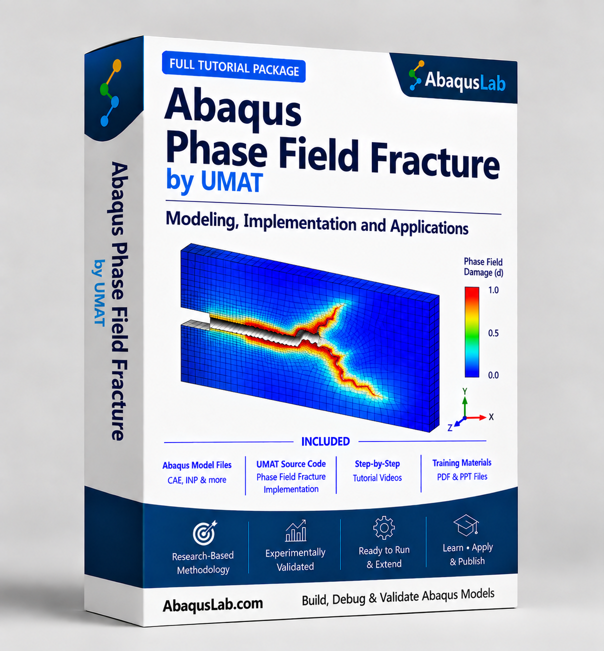

Description
Abaqus Phase Field Fracture Tutorial | UMAT & Drucker–Prager Modeling
This research-based Abaqus Phase Field Tutorial package provides a complete Abaqus Phase Field Fracture workflow for engineers and researchers. Phase Field Modeling in Abaqus requires an advanced fracture formulation. The Abaqus Phase Field formulation is implemented through an Abaqus UMAT Phase Field approach, enabling crack nucleation and propagation to be modeled without explicitly tracking the crack surface.
The methodology is based on the peer-reviewed publication in Theoretical and Applied Fracture Mechanics (2022). The formulation addresses asymmetric tensile–compressive fracture behaviour and extends phase-field fracture to pressure-sensitive brittle and quasi-brittle materials such as concrete, rock, and other geomaterials.
Rather than providing only a finished Abaqus Phase Field Fracture model, this tutorial explains the theoretical formulation, strain-energy decomposition, Drucker–Prager failure surface, Abaqus UMAT Phase Field implementation, heat-transfer analogy, material parameters, meshing strategy, crack evolution, and post-processing workflow required to understand and modify the model for your own research.
What Is Abaqus Phase Field Fracture Modeling?
Abaqus Phase Field Fracture modeling predicts crack nucleation and propagation by representing a sharp crack with a continuous phase-field variable instead of explicitly tracking the crack surface.
The phase-field variable progressively changes from the intact material state toward the fractured state, allowing complex crack paths, crack initiation, branching, merging, and propagation to develop naturally through the finite element solution.
AbaqusLab implements Phase Field Modeling in Abaqus using a research-based UMAT formulation that incorporates a Drucker–Prager-informed strain-energy decomposition for asymmetric tension–compression fracture.
The approach is particularly relevant to brittle and quasi-brittle materials whose compressive strength can differ substantially from their tensile strength and whose fracture behaviour depends on pressure, confinement, friction, and multi-axial stress conditions.
Core Abaqus Phase Field Modeling Concepts
- Abaqus Phase Field — Abaqus Phase Field modeling replaces a discrete crack surface with a regularised continuous field that evolves between intact and fractured material states.
- Abaqus Phase Field Fracture — Abaqus Phase Field Fracture predicts crack nucleation and propagation without prescribing the final crack trajectory in advance.
- Abaqus Phase Field Tutorial — the tutorial explains the complete workflow from fracture theory and strain-energy decomposition to Abaqus implementation, solution, and result interpretation.
- Phase Field Modeling in Abaqus — the mechanical equilibrium and phase-field evolution equations are solved within a coupled finite element framework.
- Abaqus UMAT Phase Field — the implementation takes advantage of the mathematical analogy between phase-field evolution and heat transfer so that the research formulation can be implemented through an Abaqus UMAT-based workflow.
- Drucker–Prager Phase Field Fracture — the fracture driving force is decomposed so that the formulation can reproduce pressure-sensitive asymmetric tensile–compressive failure.
- Abaqus Phase Field Concrete Fracture — the methodology can represent fracture under uniaxial and confined compression in quasi-brittle concrete.
- Abaqus Phase Field Geomaterials — the formulation addresses shear, friction, dilatancy, confinement, and localised failure in pressure-sensitive geomaterials.
What You Can Predict with Abaqus Phase Field Fracture
The Abaqus UMAT Phase Field formulation extends beyond a simple tensile crack example. It is designed to investigate fracture under pressure-sensitive and multi-axial loading conditions where conventional tension–compression symmetric phase-field formulations may provide unrealistic predictions.
- Crack nucleation under complex stress states
- Crack propagation without a predefined crack trajectory
- Tension–compression asymmetric fracture
- Pressure-sensitive material failure
- Frictional shear response
- Dilatancy under shear loading
- Confinement effects in brittle and quasi-brittle materials
- Concrete fracture patterns
- Geomaterial and soil failure
- Complex multi-axial cracking
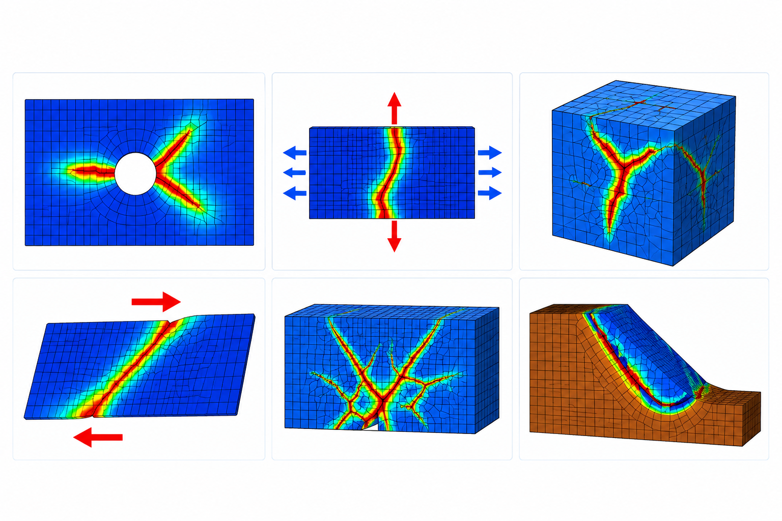
- Research-backed capability: the underlying study demonstrates phase-field predictions for shear deformation, direct shear loading, confined and unconfined concrete compression, and localised soil-slope failure.
What You Will Learn in This Abaqus Phase Field Tutorial
This Abaqus Phase Field Tutorial takes you through the complete workflow required to understand, build, run, and interpret the phase-field fracture model.
- 📘 Understand the theoretical formulation — phase-field fracture, Griffith energy, regularisation, and crack evolution.
- 🧠 Understand tension–compression asymmetry and why it matters for brittle and quasi-brittle failure.
- 📐 Derive the strain-energy decomposition associated with the fracture-driving force.
- ⚙️ Understand the Drucker–Prager failure surface and its role in pressure-sensitive fracture.
- 💻 Understand the Abaqus UMAT Phase Field implementation and the Fortran source-code structure.
- 🌡️ Understand the heat-transfer analogy used for the phase-field evolution equation.
- 🔬 Configure the Abaqus model including material parameters, fracture properties, boundary conditions, loading, and meshing.
- 📈 Study crack nucleation and propagation under different mechanical loading conditions.
- 📊 Interpret phase-field contours and analyse fracture evolution during the simulation.
- 🛠️ Adapt the supplied Abaqus models for your own material, geometry, research project, or engineering application.
By the end of the package, you will have a reusable Abaqus Phase Field Fracture workflow that can be modified for other pressure-sensitive brittle and quasi-brittle fracture problems.
What You Receive with This Abaqus Phase Field Package
This Abaqus Phase Field package is designed to provide more than a finished UMAT. You receive the complete Abaqus models, source code, step-by-step tutorial material, theoretical formulation, verification examples, and support required to understand and modify the simulation.
Complete Step-by-Step Tutorial Videos
Models, UMAT, Documentation & Support
Package objective: the goal is not only to provide working Abaqus files, but to give you a complete and reusable Abaqus UMAT Phase Field workflow that you can understand, verify, modify, and extend for your own fracture mechanics research and engineering applications.
Phase Field Modeling in Abaqus — Complete Workflow
Reliable Phase Field Modeling in Abaqus requires considerably more than simply compiling a Fortran subroutine.
The theoretical formulation, material definition, phase-field length scale, mesh resolution, boundary conditions, solution procedure, state variables, and post-processing strategy must all be defined consistently.
The Tutorial Covers
- 📘 Understand phase-field fracture theory — Griffith fracture, regularisation, crack-surface representation, and fracture-energy minimisation.
- 📐 Understand strain-energy decomposition — identify degraded and stored energy contributions controlling fracture.
- ⚙️ Implement the Drucker–Prager formulation — introduce pressure-sensitive tensile–compressive fracture behaviour.
- 💻 Implement the Abaqus UMAT — understand the material subroutine and numerical implementation step by step.
- 🌡️ Use the phase-field heat-transfer analogy — connect phase-field evolution to the Abaqus solution procedure.
- 🔒 Enforce damage irreversibility — implement and understand the phase-field history variable.
- 🔬 Select the phase-field length scale and mesh — understand the connection between ℓ and spatial discretisation.
- 📊 Post-process fracture results — visualise phase-field contours and evaluate crack initiation and propagation.
- 🛠️ Adapt the supplied Abaqus models — modify material properties, geometry, loading, and failure parameters for your own application.
By the end of the tutorial, you will have a reusable Phase Field Modeling in Abaqus workflow that can be studied, modified, and extended for other brittle and quasi-brittle fracture problems.
Abaqus UMAT Phase Field Implementation
The Abaqus UMAT Phase Field implementation is one of the most important practical aspects of this tutorial. The governing phase-field evolution equation has a mathematical structure analogous to a heat-transfer equation. This analogy enables the coupled mechanical–fracture problem to be implemented in Abaqus through a UMAT-based strategy.
The tutorial explains how the mechanical response, strain-energy decomposition, phase-field degradation, fracture driving force, history variables, and Abaqus analysis procedure work together within the numerical implementation.
- UMAT — implements the constitutive response and phase-field fracture formulation.
- Heat-transfer analogy — allows the phase-field governing equation to be solved using Abaqus thermal degrees of freedom.
- History field — stores the maximum fracture-driving energy required to enforce damage irreversibility.
- Phase-field variable — represents the local evolution from intact material to fractured material.
- Consistent Abaqus model — couples the mechanical and phase-field solutions within the finite element analysis.
If you require modification or development of another user-material formulation, AbaqusLab also provides
UMAT Consulting & Development
and
Abaqus User Subroutine Development.
Why Use Abaqus Phase Field Fracture?
The principal advantage of Abaqus Phase Field Fracture is that the crack path does not need to be explicitly tracked during the analysis. Instead, a continuous phase-field variable represents the transition between intact and fractured material. This makes phase-field fracture particularly suitable for simulations involving complex or initially unknown crack trajectories. Crack nucleation, propagation, branching, interaction, and merging can emerge from the governing equations rather than being prescribed using a predefined crack-growth path.
For engineering materials subjected to complex multi-axial loading, the method provides a powerful framework for studying the complete fracture process from the initiation of localised damage to development of a macroscopic crack.
Key advantage: Phase-field fracture replaces explicit crack tracking with a regularised fracture field, allowing complex crack evolution to be captured within a unified finite element formulation.
Abaqus Phase Field — Variational Fracture Formulation
The Abaqus Phase Field formulation used in this tutorial is based on the variational phase-field framework for fracture mechanics. The total energy of the system contains the elastic strain energy stored in the body together with the energy required to create new fracture surfaces. Instead of representing the crack as a discrete discontinuity, the sharp crack is regularised over a finite region using the phase-field variable φ.
In the conventional formulation:
- φ = 0 represents intact material.
- φ = 1 represents the fully fractured state.
- 0 < φ < 1 represents the regularised transition region around the crack.
The formulation introduces the fracture toughness Gc and the phase-field length scale ℓ. The length scale controls the width of the regularised fracture zone and therefore has an important relationship with the required finite element mesh resolution.
This regularisation allows fracture to be described through a partial differential equation governing the evolution of the phase-field variable.
Phase Field Tension–Compression Asymmetry
A major challenge in conventional phase-field fracture is its treatment of tensile and compressive loading. In a conventional Griffith-based formulation, the elastic strain-energy density can drive phase-field evolution without sufficiently distinguishing whether the local mechanical state is tensile or compressive. For brittle and quasi-brittle materials, this can lead to unrealistic predictions because tensile and compressive fracture behaviour can be fundamentally different.
The research framework implemented in this Abaqus Phase Field Tutorial addresses this limitation by decomposing the elastic strain-energy density into:
- Damage-degraded strain energy — the contribution responsible for driving fracture evolution.
- Stored non-degraded strain energy — the residual contribution that remains independent of the evolving phase-field damage.
This separation makes it possible to construct the fracture driving force according to a chosen failure criterion and therefore reproduce asymmetric tension–compression behaviour under complex multi-axial stress states.
Drucker–Prager Phase Field Fracture
The key technical feature of this package is the implementation of a Drucker–Prager Phase Field Fracture formulation. The Drucker–Prager criterion is a pressure-sensitive failure criterion commonly associated with materials such as concrete, rock, soils, foams, and other materials whose strength depends strongly on hydrostatic pressure. The failure surface is expressed using stress invariants and is characterised through parameters related to the material tensile and compressive strengths.
Instead of adding the Drucker–Prager criterion as an independent failure trigger, the underlying research framework derives the phase-field strain-energy decomposition so that the fracture formulation itself reproduces the selected Drucker–Prager failure surface.
This provides a systematic connection between:
- phase-field fracture mechanics
- strain-energy decomposition
- tensile and compressive strength
- pressure-sensitive failure
- friction and cohesion
- multi-axial stress states
Research significance: the formulation goes beyond conventional tension–compression symmetric phase-field fracture by constructing the fracture driving force so that it is compatible with a pressure-sensitive Drucker–Prager failure surface.
Abaqus Phase Field Concrete Fracture
One important application of the formulation is Abaqus Phase Field Concrete Fracture. Concrete exhibits strongly different tensile and compressive strengths and its fracture behaviour can be significantly influenced by confinement. This makes pressure-sensitive phase-field formulations particularly relevant. The reference research applies the Drucker–Prager-based phase-field formulation to concrete specimens under both uniaxial and triaxial compression.
The numerical results demonstrate that confinement increases the predicted critical load and produces a different fracture pattern compared with the unconfined specimen. The unconfined case develops a crack originating near the specimen boundary and progressing toward the centre, while the confined specimen develops an internal fracture pattern characteristic of a different stress state.
This example demonstrates why the representation of pressure sensitivity and tension–compression asymmetry is important when applying phase-field fracture to concrete and other quasi-brittle materials.
Abaqus Phase Field Geomaterials
The formulation is also particularly relevant to Abaqus Phase Field Geomaterials such as rock and soil, where fracture can depend strongly on pressure, friction, cohesion, and dilatancy.
The research investigates several examples designed to evaluate these effects.
Single-Element Shear Test
A single element is subjected to shear deformation and different levels of pressure to investigate frictional behaviour and dilatancy.
The results demonstrate how the Drucker–Prager parameter influences shear resistance and volumetric deformation as the phase-field fracture variable evolves.
Virtual Direct Shear Test
A direct shear test is simulated under different vertical pressure levels.
The phase-field results show that the applied pressure affects both the load-carrying response and predicted crack trajectory.
Localised Soil-Slope Failure
The methodology is also applied to a soil-slope stability problem.
The Drucker–Prager-based strain-energy decomposition produces a localised fracture path propagating from the foundation region toward the slope boundary and is compared with alternative phase-field strain-energy decomposition methods.
Abaqus Phase Field Crack Propagation
Abaqus Phase Field Crack Propagation is represented through the evolution and localisation of the phase-field variable rather than through explicit movement of a discrete crack tip. As the fracture driving force increases, the phase-field variable evolves from its intact state and begins to localise into a narrow fracture zone. Once localisation develops, the fracture zone can propagate naturally through the finite element mesh according to the material properties, stress state, fracture energy, and governing phase-field equations.
This approach is especially valuable when:
- the crack path is not known beforehand,
- multiple cracks can nucleate,
- cracks can branch or merge,
- complex multi-axial stresses determine the fracture direction, or
- explicit crack tracking would become difficult.
Why Abaqus Phase Field Modeling Is Challenging
A reliable Abaqus Phase Field simulation requires the fracture theory and numerical implementation to work together consistently.
Common challenges include:
- Fracture driving-force definition — incorrect strain-energy decomposition can produce unrealistic cracking.
- Tension–compression treatment — pressure-sensitive materials cannot always be represented using simple symmetric degradation.
- UMAT implementation — the constitutive equations, history variables, and coupling must be coded correctly.
- Length-scale selection — the phase-field length scale influences the regularised fracture zone.
- Mesh sensitivity — the mesh must resolve the phase-field length scale adequately.
- Convergence — progressive fracture introduces strong nonlinearities into the solution.
- Boundary conditions — mechanical and phase-field boundary conditions must be defined consistently.
- Result interpretation — phase-field contours must be understood correctly when identifying crack initiation and propagation.
The objective of this Abaqus Phase Field Tutorial is therefore not simply to provide a model that runs, but to explain the theory and implementation so that the workflow can be understood, verified, and adapted.
Research-Based Abaqus Phase Field Validation
The methodology is based on the peer-reviewed paper:
Y. Navidtehrani, C. Betegón and E. Martínez-Pañeda,
A General Framework for Decomposing the Phase Field Fracture Driving Force, Particularised to a Drucker–Prager Failure Surface,
Theoretical and Applied Fracture Mechanics 121 (2022) 103555.
Read the peer-reviewed Phase Field Fracture paper →
The study presents a general methodology for decomposing the phase-field fracture driving force according to an arbitrary failure criterion and then particularises that methodology to a Drucker–Prager failure surface.
The numerical implementation is evaluated through four representative groups of simulations:
- Single-element shear deformation — friction and dilatancy effects.
- Virtual Direct Shear Tests — pressure-dependent fracture and crack trajectories.
- Concrete compression — uniaxial and triaxial confinement effects.
- Soil-slope failure — localised failure and comparison with alternative energy decompositions.
The published results demonstrate the capability of the formulation to reproduce crack nucleation and growth under multi-axial loading in materials exhibiting asymmetric tensile–compressive fracture behaviour.
Scientific basis: this package translates a peer-reviewed Drucker–Prager phase-field fracture framework into a practical Abaqus learning and implementation workflow rather than relying on an undocumented empirical fracture model.
Who Is This Abaqus Phase Field Tutorial For?
This package is designed for researchers and engineers who want to understand and implement advanced phase-field fracture mechanics rather than simply use a black-box Abaqus model.
- PhD and MSc researchers working on fracture mechanics and computational mechanics.
- Researchers studying phase-field fracture and crack nucleation or propagation.
- Concrete researchers investigating brittle and quasi-brittle failure.
- Rock and geomaterial researchers studying pressure-dependent fracture.
- Abaqus users developing UMAT subroutines for advanced constitutive and fracture formulations.
- Engineers studying complex crack paths where the fracture trajectory is not known beforehand.
- Researchers studying confinement and multi-axial failure.
Basic knowledge of finite element analysis and Abaqus is recommended. The tutorial is intended to explain the implementation sufficiently clearly that users can understand the formulation even if they have limited previous experience with phase-field programming.
Explore More Advanced Abaqus Modeling Tutorials
Beyond Abaqus Phase Field Fracture, AbaqusLab provides advanced simulation packages covering constitutive modeling, fracture mechanics, multiphysics, and custom user-subroutine development.
Explore our related tutorial collections:
Crystal Plasticity in Abaqus,
Peridynamics in Abaqus,
and
Abaqus Hydrogen Modeling.
Frequently Asked Questions
What is Abaqus Phase Field?
Abaqus Phase Field modeling represents fracture using a continuous field variable instead of explicitly representing a sharp crack surface. The phase-field variable evolves from the intact state toward the fractured state as crack nucleation and propagation occur.
What is Abaqus Phase Field Fracture?
Abaqus Phase Field Fracture is a finite element fracture approach that allows cracks to nucleate and propagate without explicitly prescribing or tracking their trajectory. Crack evolution is determined through the coupled mechanical and phase-field governing equations.
How is Phase Field Modeling implemented in Abaqus?
In this package, Phase Field Modeling in Abaqus uses the mathematical analogy between the phase-field evolution equation and heat transfer. The research formulation is implemented using an Abaqus UMAT-based approach.
What is Abaqus UMAT Phase Field?
Abaqus UMAT Phase Field refers to the custom user-material implementation used to define the mechanical constitutive response, strain-energy decomposition, fracture-driving quantities, degradation behaviour, and history-dependent variables required by the phase-field formulation.
What is Drucker–Prager Phase Field Fracture?
Drucker–Prager Phase Field Fracture incorporates a pressure-sensitive failure surface into the phase-field fracture driving-force formulation. It is particularly useful for brittle and quasi-brittle materials with different tensile and compressive strengths.
Why is tension–compression asymmetry important?
Many brittle and quasi-brittle materials have significantly different tensile and compressive strengths. A fracture formulation that does not distinguish sufficiently between these states can predict unrealistic crack initiation. The strain-energy decomposition used here is designed to account for this asymmetry.
Can Abaqus Phase Field model concrete fracture?
Yes. The underlying research formulation includes simulations of concrete under uniaxial and triaxial compression and investigates how confinement influences predicted strength and fracture patterns.
Can Abaqus Phase Field be used for geomaterials?
Yes. The formulation is especially relevant to pressure-sensitive geomaterials. The reference research includes shear deformation, direct shear tests, and localised soil-slope failure.
Does phase-field fracture require a predefined crack path?
No. One of the principal advantages of phase-field fracture is that the crack path evolves through the numerical solution and therefore does not generally need to be prescribed in advance.
What is the phase-field length scale?
The phase-field length scale ℓ controls the width of the regularised fracture region. The finite element mesh must provide sufficient resolution relative to this length scale for reliable representation of the phase-field solution.
Why is mesh refinement important in Abaqus Phase Field simulations?
The phase-field variable changes rapidly across the regularised fracture region. If the mesh is too coarse relative to the phase-field length scale, the fracture field and predicted crack behaviour may not be resolved adequately.
What does the history field do?
The history field stores the maximum value of the relevant fracture-driving energy during the loading history. It is used to enforce damage irreversibility and prevent an already fractured material point from artificially recovering.
Can I modify the supplied UMAT for my own research?
The package is designed to explain the formulation and implementation so that researchers can understand and adapt the supplied workflow. Any modified implementation should be independently verified and validated for the specific material, geometry, and loading conditions.
Do you provide custom Abaqus Phase Field project support?
Yes. AbaqusLab provides custom phase-field model development, UMAT development, debugging, verification, validation, and advanced Abaqus consulting for research and engineering projects.
Need a Custom Abaqus Phase Field Model?
If your project requires a different material, geometry, loading condition, fracture criterion, phase-field formulation, or custom UMAT implementation, AbaqusLab can develop and validate a dedicated Abaqus workflow for your application.
Our
Abaqus Consulting
service supports advanced finite element model development, while
UMAT Consulting
and
Abaqus User Subroutine Development
support custom constitutive and numerical formulations.
For convergence problems, existing-model errors, or implementation troubleshooting, visit
Abaqus Help & Technical Support.
Start Learning Abaqus Phase Field Fracture
Use this complete Abaqus Phase Field Tutorial to understand the theory, study the Drucker–Prager formulation, implement the Abaqus UMAT Phase Field workflow, and build reliable phase-field fracture simulations for your own research or engineering applications.



Reviews
There are no reviews yet.