
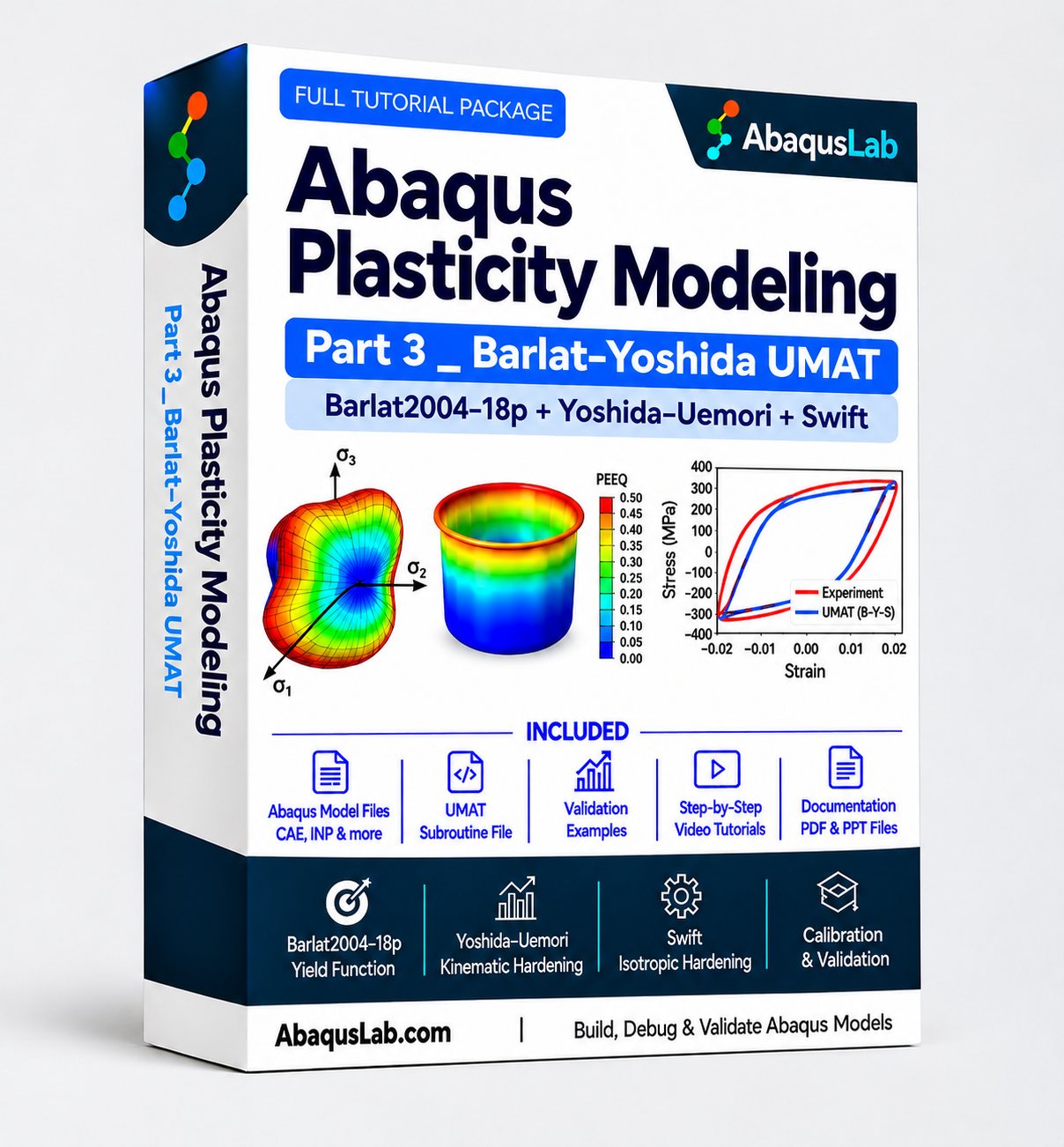


Description
Abaqus Barlat Yoshida UMAT Tutorial | Advanced Anisotropic Plasticity
This Abaqus Barlat Yoshida UMAT tutorial introduces advanced Abaqus Anisotropic Plasticity modeling in Abaqus/Standard by combining the Barlat2004-18p UMAT for directional yielding with the Yoshida Uemori UMAT for cyclic plasticity and the Bauschinger effect. The formulation is further enhanced by the Abaqus Swift Hardening Model to capture isotropic hardening and material strength evolution. Through practical Fortran implementation and Abaqus simulations, you will learn to evaluate anisotropic stress–strain behavior under monotonic and cyclic loading.
What Is Abaqus Barlat Yoshida UMAT and How Does Advanced Anisotropic Plasticity Work?
Abaqus Barlat Yoshida UMAT is a user-defined material implementation for Abaqus/Standard that combines the Barlat2004-18p anisotropic yield function, Yoshida–Uemori kinematic hardening, and Swift isotropic hardening. It is used to study direction-dependent plastic yielding and evolving material response under monotonic, unloading, reverse, or cyclic deformation. In this tutorial, Abaqus Anisotropic Plasticity is modeled through Fortran UMAT source code and finite element simulations.
What Does the Barlat2004-18p UMAT Model?
The Barlat2004-18p UMAT introduces an anisotropic yield criterion with 18 material coefficients in its common three-dimensional formulation. It captures direction-dependent yielding more flexibly than isotropic von Mises plasticity. The yield function defines when plastic flow begins; its derivatives are used to calculate plastic flow direction in an associated-flow implementation. Parameters must be calibrated for the material and its directional response.
How Does Yoshida Uemori UMAT Describe Kinematic Hardening and the Bauschinger Effect?
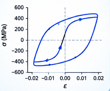
A Yoshida Uemori UMAT represents nonlinear kinematic hardening through evolving backstress variables. This helps describe the Bauschinger effect, transient hardening, and stress reversal during loading–unloading–reloading. It is particularly relevant to sheet-metal forming and springback studies, where material response depends on deformation history. Exact backstress evolution equations depend on the implementation.
What Is the Abaqus Swift Hardening Model and Why Combine It with Yoshida–Uemori?
The Abaqus Swift Hardening Model describes the evolution of isotropic flow stress with accumulated plastic strain, often written as a power law. In the combined Abaqus Barlat Yoshida UMAT, Swift hardening controls the expansion of the flow-strength scale while Yoshida–Uemori controls translation and evolution of the yield surface through backstress. The combination can represent both directional yielding and deformation-history effects.
How Is Abaqus Anisotropic Plasticity Implemented with a Fortran UMAT?
In Abaqus Anisotropic Plasticity modeling, the Fortran UMAT receives strain increments and material state information, evaluates the anisotropic yield condition, updates stress and hardening variables, and returns the material Jacobian DDSDDE to Abaqus/Standard. A reliable implementation requires consistent tensor conventions, stable constitutive integration, and verification under different loading directions and loading reversals.
When Should Engineers Use Barlat–Yoshida Instead of Hill48 or von Mises Plasticity?
Use Barlat2004-18p UMAT when a more flexible anisotropic yield surface is needed, particularly for materials with significant directional plastic response. Hill48 provides a simpler quadratic anisotropic yield criterion, while von Mises assumes isotropic yielding. Combining Barlat2004-18p with Yoshida Uemori UMAT and Abaqus Swift Hardening Model adds hardening behavior relevant to reverse loading and springback. Model choice depends on available calibration data and verification needs.
Barlat2004-18p, Yoshida–Uemori and Swift UMAT — Constitutive Model and Governing Equations
The combined Abaqus Barlat Yoshida UMAT uses an anisotropic yield function and two complementary hardening descriptions. The expressions below are illustrative constitutive relationships for explaining the model; coefficient definitions, normalizations, evolution laws, and numerical integration details must be matched to the actual Fortran source code before treating them as exact implementation equations.
1. Combined Constitutive Framework
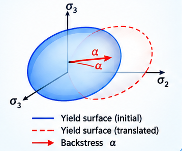
Plastic flow is governed by an anisotropic yield function, an evolving backstress, and an isotropic hardening scale.
f(\boldsymbol{\sigma},\boldsymbol{\alpha},\bar\varepsilon^p)=\Phi_{\mathrm{Barlat2004}}(\boldsymbol{\sigma}-\boldsymbol{\alpha})-Y_{\mathrm{Swift}}(\bar\varepsilon^p)\leq 0
\]
- Anisotropic yield function: Barlat2004-18p
- Kinematic hardening: Yoshida–Uemori
- Isotropic hardening: Swift
- Fortran UMAT in Abaqus/Standard
2. Barlat2004-18p Yield Criterion
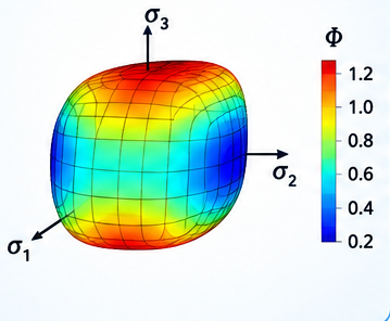
Two linearly transformed stress tensors and 18 anisotropy parameters are used in the common three-dimensional Barlat2004-18p formulation.
\Phi_{\mathrm{Barlat2004}}=\Phi(\mathbf L^{\prime}:\mathbf s,\mathbf L^{\prime\prime}:\mathbf s;\mathbf a,m)
\]
3. Yoshida–Uemori Kinematic Hardening
Backstress variables describe translation and evolution of the yield surface under plastic deformation and reversal.
\boldsymbol{\sigma}_{\mathrm{eff}}=\boldsymbol{\sigma}-\boldsymbol{\alpha}
\]
- Nonlinear kinematic hardening
- Bauschinger effect
- Unloading and reverse loading
- Transient hardening and springback-related behavior
4. Swift Isotropic Hardening
A commonly used Swift power law relates the flow-stress scale to accumulated equivalent plastic strain.
Y_{\mathrm{Swift}}=K(\varepsilon_0+\bar\varepsilon^p)^n
\]

5. Plastic Flow and Stress Integration
For an associated plasticity formulation, the plastic strain increment follows the normal to the anisotropic yield surface.
\Delta\boldsymbol{\varepsilon}^{p}=\Delta\lambda\,\frac{\partial f}{\partial\boldsymbol{\sigma}}
\]
The local constitutive update solves for plastic increments and state variables; nonlinear iteration and convergence checks are central to numerical robustness.

6. UMAT State Variables and DDSDDE
The Abaqus/Standard UMAT updates the stress vector, material state variables, and constitutive tangent.
\mathrm{STRESS}_{n+1},\quad\mathrm{STATEV}_{n+1},\quad\mathrm{DDSDDE}
\]
- Plastic strain and equivalent plastic strain
- Backstress and hardening history
- Consistent tensor ordering and shear convention
- Jacobian consistency and convergence checks

7. Directional Plasticity and Calibration
Directional tests help identify the anisotropy coefficients; reverse-loading tests inform kinematic hardening parameters.
- Uniaxial tests at multiple orientations
- Yield stresses and, where available, plastic strain ratios
- Reverse loading / tension–compression data
- Swift hardening parameter calibration

8. Typical Abaqus Results and Verification
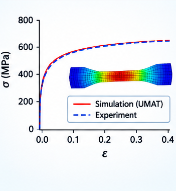
Useful output includes stress–strain curves, equivalent plastic strain, backstress-related state variables, and unloading–reloading response.
- Single-element constitutive verification
- Directional stress–strain comparisons
- Bauschinger and cyclic response checks
- Mesh, increment, and convergence sensitivity
Recommended Prerequisite for Barlat2004-18p UMAT — Plasticity Part 2
Learn Abaqus UMAT Fundamentals Before Advanced Anisotropic Plasticity
Part 2 builds on the Fortran programming, UMAT interface, stress-update algorithms, and state-variable foundations covered in Part 1. The Abaqus UMAT Tutorial | Essential Fundamentals for Plasticity is recommended for newcomers to user-defined constitutive modeling; experienced UMAT developers may study Part 3 independently.
Recommended learning sequence:
What Does the Abaqus Barlat Yoshida UMAT Tutorial Cover?
This Abaqus Barlat Yoshida UMAT tutorial connects the Barlat2004-18p UMAT anisotropic yield surface, Yoshida Uemori UMAT backstress evolution, and Abaqus Swift Hardening Model with practical Fortran implementation and Abaqus Anisotropic Plasticity simulations.
Barlat2004-18p UMAT
Advanced anisotropic yield-surface formulation and directional plasticity.
Yoshida Uemori UMAT
Nonlinear kinematic hardening and backstress evolution.
Abaqus Swift Hardening Model
Isotropic hardening and plastic strain-dependent flow strength.
Abaqus Anisotropic Plasticity
Directional yield behavior and material coefficient interpretation.
Bauschinger Effect
Reverse-loading and loading-history-dependent plasticity.
Fortran UMAT Implementation
Material properties, STRESS, STATEV and DDSDDE.
Constitutive Integration
Plastic correction, iterative solution and numerical stability.
Anisotropy Calibration
Directional stress response and material parameter identification.
Cyclic Loading Response
Unloading, reloading and reverse plastic deformation.
Springback-Relevant Hardening
Backstress evolution relevant to unloading response.
Single-Element Verification
Checks on yield response, tangent and state updates.
Results Interpretation
Stress–strain curves, plastic strain and hardening response.
Abaqus Plasticity Modeling Learning Paths & Recommended Packages — Parts 1–8
The AbaqusLab Plasticity Modeling Series begins with Part 1 — UMAT fundamentals for static/implicit plasticity and Part 2 — VUMAT fundamentals for dynamic/explicit plasticity. Select advanced tutorials based on your application: Barlat–Yoshida–Swift (Part 3), Hill48 (Part 4), Johnson–Cook UMAT (Part 5), Johnson–Cook VUMAT (Part 6), Unified Viscoplasticity for Ti-6Al-4V (Part 7), or Overstress & Cap Viscoplasticity (Part 8). Recommended approach: Choose Part 1 for UMAT applications or Part 2 for VUMAT applications, then add the advanced parts you need. Each advanced tutorial may also be purchased independently.
Part 1 — Abaqus UMAT Fundamentals for Static Plasticity
- 🔹 Abaqus UMAT subroutine fundamentals
- 🔹 Fortran programming and UMAT implementation
- 🔹 Plasticity constitutive equations
- 🔹 Return mapping, debugging and validation
Part 2 — Abaqus VUMAT Fundamentals for Dynamic Plasticity
- 🔹 Abaqus VUMAT and Fortran fundamentals
- 🔹 Abaqus/Explicit material modeling
- 🔹 Stress updates and state variables
- 🔹 Foundation for advanced VUMAT tutorials
Parts 1 + 2
UMAT & VUMAT Fundamentals
Learn Abaqus/Standard and Abaqus/Explicit user-material programming.
Part 3 — Barlat–Yoshida–Swift Plasticity UMAT
- 🔹 Barlat2004-18p anisotropic yield function
- 🔹 Yoshida–Uemori kinematic hardening
- 🔹 Swift isotropic hardening
- 🔹 Advanced UMAT implementation
Build Your Own AbaqusLab Bundle
- Search all eligible tutorials and select any combination.
- Save 25% with 2 tutorials, with discounts increasing up to 55% for 8 or more.
- See your bundle total instantly and proceed to WooCommerce check0ut.
Part 4 — Hill48 Anisotropic Plasticity UMAT
- 🔹 Hill48 anisotropic yield criterion
- 🔹 Hill48 UMAT Fortran implementation
- 🔹 Directional plasticity and anisotropy
- 🔹 Stress–strain response and validation
Part 5 — Johnson–Cook Plasticity UMAT
- 🔹 Johnson–Cook constitutive formulation
- 🔹 Strain-rate-dependent plasticity
- 🔹 Temperature-dependent material behavior
- 🔹 UMAT implementation in Abaqus/Standard
Part 6 — Johnson–Cook Plasticity VUMAT
- 🔹 Johnson–Cook constitutive formulation
- 🔹 Explicit dynamic material modeling
- 🔹 High-strain-rate deformation
- 🔹 VUMAT stress updates and state variables
Part 7 — Unified Viscoplasticity UMAT — Ti-6Al-4V
- 🔹 Ti-6Al-4V hot forming
- 🔹 Microstructure-based viscoplasticity
- 🔹 Dislocation evolution and globularisation
- 🔹 Phase transformation and thermal softening
Part 8 — Viscoplasticity UMAT — Overstress & Cap Plasticity
- 🔹 Overstress-based viscoplastic flow
- 🔹 Pressure-sensitive yield surfaces
- 🔹 Tensile cutoff and cap plasticity
- 🔹 Implicit stress integration
Parts 1 + 3 + 4
UMAT + Barlat–Yoshida + Hill48
For anisotropic metals, sheet forming, and advanced hardening models.
Parts 2 + 6
VUMAT + Johnson–Cook Plasticity
For explicit dynamic modeling and user-defined Johnson–Cook material behavior.
Parts 1 + 7 + 8
UMAT + Two Viscoplasticity Models
For rate-dependent constitutive models and hot-forming applications.
Build the Full Abaqus Plasticity Bundle — Parts 1–8
- UMAT and VUMAT fundamentals
- Barlat–Yoshida–Swift and Hill48 anisotropic plasticity
- Johnson–Cook plasticity in Abaqus/Standard and Abaqus/Explicit
- Unified viscoplasticity for Ti-6Al-4V hot forming
- Overstress & cap viscoplasticity
- All eight numbered tutorials in one package
What You Receive with This Abaqus Barlat Yoshida UMAT Tutorial
This Abaqus Barlat Yoshida UMAT learning package is intended to help you understand, run, and adapt the combined Barlat2004-18p UMAT, Yoshida Uemori UMAT, and Abaqus Swift Hardening Model workflow. The package centers on the existing Fortran subroutine and Abaqus simulation files, together with step-by-step teaching materials. Confirm the precise downloadable file list and support terms against your final product package before publishing.
Complete Barlat–Yoshida UMAT Tutorial Videos
UMAT Source Code, Abaqus Models & Supporting Materials
Abaqus Barlat Yoshida UMAT Tutorial — Learning Sequence
Abaqus Anisotropic Plasticity — UMAT Simulation and Verification Workflow
The Abaqus Barlat Yoshida UMAT workflow connects material identification, Fortran programming, Abaqus/Standard setup, and numerical validation. The steps below provide a practical checklist for using the combined model.
What You Will Learn with the Abaqus Barlat Yoshida UMAT Tutorial
Understand Barlat2004-18p UMAT
Interpret directional yielding and anisotropic coefficients.
Implement Yoshida Uemori UMAT
Understand nonlinear backstress evolution and reverse loading.
Use Abaqus Swift Hardening Model
Relate accumulated plastic strain to isotropic flow stress.
Build Abaqus Anisotropic Plasticity Models
Configure material properties, boundary conditions, and output.
Interpret the Bauschinger Effect
Study how prior plastic deformation affects reversed yielding.
Read and Adapt Fortran UMAT Code
Understand UMAT variables, state storage, and tangent stiffness.
Validate Plasticity Constitutive Response
Compare yield, hardening, and stress–strain trends.
Apply Advanced Material Modeling
Prepare for sheet-metal plasticity and springback-oriented studies.
Who Is This Abaqus Barlat Yoshida UMAT Tutorial For?
- Researchers developing anisotropic plasticity constitutive models
- Engineers analyzing sheet-metal deformation and directional yielding
- Finite element analysts working with Abaqus/Standard UMAT
- MSc and PhD students studying Barlat2004-18p plasticity
- Researchers investigating Yoshida–Uemori hardening and Bauschinger effects
- Fortran developers implementing combined isotropic–kinematic hardening
- Engineers evaluating Swift hardening and unloading behavior
Need Custom Abaqus Anisotropic Plasticity or UMAT Development?
Advanced Abaqus Anisotropic Plasticity often requires calibration of Barlat2004-18p UMAT coefficients, Yoshida Uemori UMAT parameters, and Abaqus Swift Hardening Model constants. AbaqusLab consulting can support custom constitutive development, model verification, and adaptation to your experimental data.
Abaqus Barlat Yoshida UMAT — Frequently Asked Questions
What is Abaqus Barlat Yoshida UMAT?
It is a combined Abaqus/Standard Fortran UMAT approach using Barlat2004-18p anisotropic yielding, Yoshida–Uemori kinematic hardening, and Swift isotropic hardening.
What does the Barlat2004-18p UMAT capture?
It represents direction-dependent plastic yielding using a flexible anisotropic yield criterion, subject to calibration of its material coefficients.
Why use Yoshida Uemori UMAT?
Yoshida–Uemori kinematic hardening helps describe backstress evolution, the Bauschinger effect, and reverse-loading behavior.
What is the Abaqus Swift Hardening Model?
Swift hardening is a power-law description of isotropic flow-stress evolution with accumulated plastic strain.
Does the tutorial use Abaqus/Standard or Abaqus/Explicit?
The UMAT formulation is intended for Abaqus/Standard. Abaqus/Explicit normally uses the separate VUMAT interface.
Is this tutorial suitable for sheet-metal springback modeling?
The constitutive framework is relevant to springback studies because anisotropy and unloading/reverse-loading hardening can matter. Specific springback benchmarks should be confirmed against the supplied simulations.
Do I need Part 1 first?
Part 1 is recommended for beginners in Fortran UMAT programming. Experienced developers may begin with Part 2.
How is Part 2 different from Hill48 Part 3?
Part 2 combines the advanced Barlat2004-18p anisotropic yield criterion with Yoshida–Uemori and Swift hardening; Part 3 focuses on Hill48 anisotropic plasticity.
What should be checked before applying the model to a new material?
Verify anisotropy coefficients, hardening parameters, stress-integration conventions, tangent stiffness, and agreement with directional and reverse-loading tests.
Related Abaqus UMAT, Plasticity, Materials Modeling & Advanced Simulation Resources
Continue from Abaqus Barlat Yoshida UMAT to Abaqus UMAT fundamentals, Hill48 anisotropic plasticity, advanced constitutive modeling, and related AbaqusLab learning paths. These internal resources help connect plasticity subroutines with calibration, fracture, and numerical simulation.
1. RELATED PLASTICITY TUTORIALS
2. PLASTICITY SUITE & AUTOMATION
3. FRACTURE & MATERIAL MODELING
4. OTHER ADVANCED MATERIAL TUTORIALS
5. CONSULTING & SUPPORT
6. EXTERNAL RESOURCES & RESEARCH
Consult official Abaqus UMAT documentation and peer-reviewed constitutive modeling research for implementation details and model calibration.


Reviews
There are no reviews yet.